An Empirical Defense of Congressional Filibusters and Super-Majority Voting Rules

Deliberative democracy is a noble ideal that politics reduces to romantic fiction. Deliberations rarely produce unanimous agreement due to the divergent interests of politicians and their constituencies. The upshot is that policy issues, both great and small, often are resolved by narrow majority votes. As the jurist and legal scholar Robert Bork noted, even scant majorities rule for no better reason than that they are majorities.

Whether a policy decision requires a simple majority (i.e., 50 percent plus one of the votes cast), or else a super-majority of some degree, should depend—at the very least—upon the significance of the policy under consideration; i.e., a vote to commemorate Groundhog Day surely is of less significance than a vote to transform American society. Regrettably, the choice of degree is itself a policy issue that typically eludes unanimous consent. That choice often follows tradition; in other instances it turns ad hoc on the whim of interested politicians. A variety of ideally objective voting schemes have been proposed by economists and political theorists (e.g., variations on “Wicksellian unanimity”), but none so far has gained widespread traction. This failure is attributable partly to the impracticality of the schemes proposed, and partly to the fact that they constrain the felicitous degree of flexibility that politicians, judges, and bureaucrats presently enjoy.

Majority voting rules in the Supreme Court and in Congress are examined empirically in the sections below.

The Supreme Court

The Supreme Court’s simple majority voting rule has captured the attention of law and economics scholars. Their concern is that transformative constitutional interpretations can (and often do) hinge on the political ideology of a single “swing” Justice. The judicial rule of stare decisis gives long life to voting errors.

The law and economics scholar Gordon Tullock addressed empirically the Supreme Court’s simple majority voting rule. [Good, I.J., and Gordon Tullock. 2004. “Judicial Errors and a Proposal for reform.” In The Selected Works of Gordon Tullock. Volume I: Virginia Political Economy, edited by C. Roley, pp. 484–494. Indianapolis: Liberty Fund.] He concluded, “in those cases where the probability is low that the court[‘s decision] is correct, that is, in the Supreme Court the five to four and six to three cases, the decisions should not be regarded as precedent.”

To explore the likelihood that a decision by the Court might be in error, Tullock and co-author, statistician I.J. Good, devised an empirical method for deriving “the subjective, logical, or epistemic probability ... that an exceedingly large court drawn at random from the infinite population will agree with the decision of the original court, that is, that the majority of the very large court will vote yes ...” Their results demonstrated, in the case of 5–4 decisions, “the possibility that the court’s decision is wrong is at least 37 percent.” Conversely, the complementary probability that the decision is correct is 63 percent (100 – 37 = 63). The probability of error predictably decreases as the majority increases: for 6–3 decisions, the probability of error falls to 27 percent; for 7–2 decisions it is 5 percent; for 8–1 decisions it is 1 percent; for 9–0 decisions, the probability of error is virtually zero.

The authors argue that “[b]oth the [judicial] reform we suggest, and our initial calculation of the probable percentage of errors by the Court, are apt to be regarded as very radical by conventional minds. The view that the Court cannot make mistakes has been widely held, although, given the number of times it has reversed itself, it is hard to see why.”

Congress

This line of reasoning extends to congressional voting schemes, yet there is little evidence that this extension has been attempted. An explanation for is lacuna might be that the probability mathematics underlying the methodology are daunting, and the calculations themselves are cumbersome when the voting body is large. Fortunately, as the authors note, “this probability is well approximated by the tail-area probability of a normal deviate equal to”

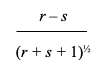
where r represents the number of majority votes, and s represents the complementary number of minority votes. In language more recognizable to the layman, relevant probabilities of truth and error are approximated by the “cumulative normal distribution”; i.e., the area under the familiar “bell curve.” These values can be read directly from standard statistical tables, and produced perfunctorily by pre-programmed spreadsheet functions. The above equation produces the required “x” values.

Estimating Congressional Voting Errors

The U.S. Constitution prescribes super-majority minimums for such issues as Constitutional amendments (75 percent) and the override of presidential vetoes (67 percent). The Senate often exercises a 60-vote super-majority “filibuster” rule, which comes under attack when scant majorities fervently desire to pass controversial legislation. The House, by contrast, has no such rule. When Senate votes are tied, the Vice President casts the deciding vote. Otherwise, simple majority rules apply in both houses. Fewer than the full complement of 100 Senators and 435 Representative often cast ballots; reduced turnouts are found to have little effect on the shape of the error probability function.

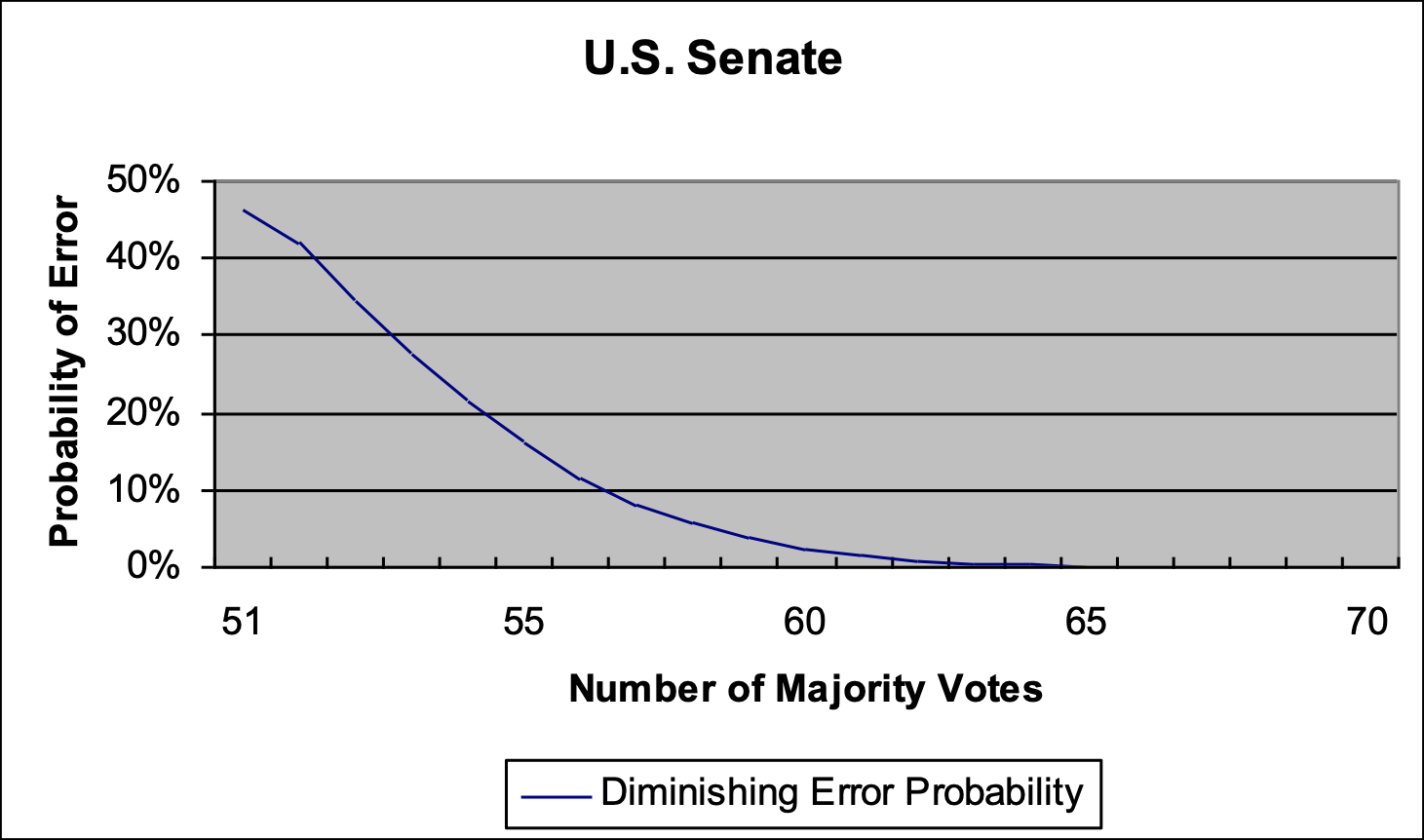
Error probabilities for Senate and House votes are depicted graphically in the two charts below; the cumulative normal distribution has been employed for ease of calculation. Error probabilities are shown on the charts’ vertical axis; the number of majority votes is shown on the horizontal axis. The resulting error probabilities imply that an infinitely large House or Senate—alternatively stated: a large number of congressional bodies, comprising and an ever-shifting mix of political ideologies voting over long time intervals—only rarely would adopt erroneous policies.

Majority Senate Voting

Error probabilities for Senate voting are depicted in the chart below. The kink in the data reflects the effect of a Vice President’s tie-breaking vote.

This chart shows, as expected, that the error probability declines as the voting majority increases. Somewhat surprising is that the error probability is 46 percent when the Vice President breaks a 50–50 tie, yet only 42 percent when the vote is 51–49. Error probability is 2 percent under the Senate’s 60-vote filibuster rule, and is virtually zero when the majority casts 65 votes.

Majority House Voting

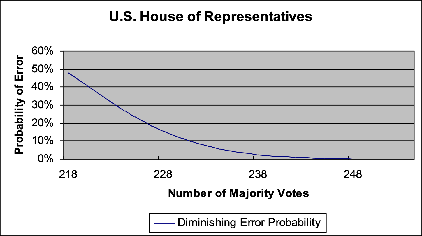
Error probabilities for House voting are depicted in the chart below.

This chart, like its predecessor, shows error probabilities declining as voting majorities increase. Here, the error probability drops from 48 percent when the vote is 218–217, to virtually zero when the majority vote rises above 248. The error probability touches 2 percent—the equivalent of a 60-vote Senate filibuster—at 239 votes.

Conclusion

Error probabilities in both the Senate and House approach zero as voting majorities increase. The Senate’s filibuster rule appears to be publicly beneficial, both because it substantially decreases the probability of error, and because it will tend to increase the level of public trust and confidence in policy outcomes when, as now, the process of deliberative democracy is in disrepute.

Any approach to re-structuring majority voting rules ironically would require a majority vote. The methodology described above outlines a means for sizing that majority, as well as others.